library(tidyverse)
library(rnaturalearth) # install if not available5 Pivoting and Joining
5.1 Overview
In this chapter, we will explore the life expectancy data across countries. Life expectancy is a key indicator of a country’s overall health and well-being. By analyzing this data, we can identify trends and disparities in life expectancy across different regions and countries.
About the data
This dataset was downloaded from the World Bank website and saved as a CSV file named life_expectancy.csv, stored in the data folder. The dataset was last updated on March 24, 2025, contains the life expectancy at birth for various countries over the years.
Learning Objectives
This chapter will demonstrate two data wrangling techniques:
- Transforming wide data to long data format using
pivot_longer(). - Merging datasets using
left_join()for map visualization.
5.2 Load data and packages
To merge the life expectancy data with the world map data, we will use the rnaturalearth package for world map data.
# Load the life expectancy data
lifex <- read_csv("data/life_expectancy.csv")
New names:
Rows: 266 Columns: 69
── Column specification
──────────────────────────────────────────────────────── Delimiter: "," chr
(4): Country Name, Country Code, Indicator Name, Indicator Code dbl (63): 1960,
1961, 1962, 1963, 1964, 1965, 1966, 1967, 1968, 1969, 1970, ... lgl (2): 2023,
...69
ℹ Use `spec()` to retrieve the full column specification for this data. ℹ
Specify the column types or set `show_col_types = FALSE` to quiet this message.
• `` -> `...69`glimpse(lifex)Rows: 266
Columns: 69
$ `Country Name` <chr> "Aruba", "Africa Eastern and Southern", "Afghanistan"…
$ `Country Code` <chr> "ABW", "AFE", "AFG", "AFW", "AGO", "ALB", "AND", "ARB…
$ `Indicator Name` <chr> "Life expectancy at birth, total (years)", "Life expe…
$ `Indicator Code` <chr> "SP.DYN.LE00.IN", "SP.DYN.LE00.IN", "SP.DYN.LE00.IN",…
$ `1960` <dbl> 64.15200, 44.09883, 32.53500, 37.84614, 38.21100, 54.…
$ `1961` <dbl> 64.53700, 44.40108, 33.06800, 38.16548, 37.26700, 55.…
$ `1962` <dbl> 64.75200, 44.76804, 33.54700, 38.73579, 37.53900, 56.…
$ `1963` <dbl> 65.13200, 44.92569, 34.01600, 39.06327, 37.82400, 57.…
$ `1964` <dbl> 65.29400, 45.49893, 34.49400, 39.33362, 38.13100, 58.…
$ `1965` <dbl> 65.50200, 45.51282, 34.95300, 39.61488, 38.49500, 60.…
$ `1966` <dbl> 66.06300, 45.26340, 35.45300, 39.83348, 38.75700, 60.…
$ `1967` <dbl> 66.43900, 45.93304, 35.92400, 39.46643, 39.09200, 61.…
$ `1968` <dbl> 66.75700, 46.22975, 36.41800, 40.07945, 39.48400, 62.…
$ `1969` <dbl> 67.16800, 46.43694, 36.91000, 40.34288, 39.82900, 63.…
$ `1970` <dbl> 67.58300, 46.72371, 37.41800, 41.02645, 40.19000, 64.…
$ `1971` <dbl> 67.97500, 47.20967, 37.92300, 41.54788, 40.55400, 65.…
$ `1972` <dbl> 68.57700, 46.91316, 38.44400, 42.24128, 40.90500, 66.…
$ `1973` <dbl> 69.09200, 47.72271, 39.00300, 42.84673, 41.27000, 67.…
$ `1974` <dbl> 69.50300, 47.63436, 39.55000, 43.48896, 41.65200, 67.…
$ `1975` <dbl> 69.76200, 47.79288, 40.10000, 44.19265, 41.19100, 68.…
$ `1976` <dbl> 70.03500, 48.37347, 40.64500, 44.99494, 41.16300, 68.…
$ `1977` <dbl> 70.26400, 48.65676, 41.22800, 45.71210, 41.43700, 69.…
$ `1978` <dbl> 70.49400, 48.78190, 40.27100, 46.26202, 41.83000, 69.…
$ `1979` <dbl> 70.77800, 49.27690, 39.08600, 46.66625, 42.17500, 69.…
$ `1980` <dbl> 71.06600, 49.65491, 39.61800, 47.00825, 42.44900, 70.…
$ `1981` <dbl> 71.72200, 50.08262, 40.16400, 47.29049, 42.77200, 70.…
$ `1982` <dbl> 71.95900, 50.33266, 37.76600, 47.52312, 43.05100, 71.…
$ `1983` <dbl> 72.10500, 48.75816, 38.18700, 47.77922, 42.09200, 71.…
$ `1984` <dbl> 72.25100, 48.71600, 33.32900, 47.92625, 42.35300, 71.…
$ `1985` <dbl> 72.38800, 49.08027, 33.55000, 48.01570, 42.64800, 71.…
$ `1986` <dbl> 72.46200, 49.71145, 39.39600, 48.06035, 42.84300, 71.…
$ `1987` <dbl> 72.78900, 50.11539, 39.84400, 48.22949, 40.91700, 72.…
$ `1988` <dbl> 73.04700, 49.37453, 43.95800, 48.50468, 41.54500, 72.…
$ `1989` <dbl> 73.02300, 50.72100, 45.15800, 48.68021, 41.76500, 72.…
$ `1990` <dbl> 73.07600, 50.64266, 45.96700, 48.63821, 41.89300, 73.…
$ `1991` <dbl> 73.10000, 50.41606, 46.66300, 48.64873, 43.81300, 73.…
$ `1992` <dbl> 73.17900, 49.97447, 47.59600, 48.72149, 42.20900, 73.…
$ `1993` <dbl> 73.22500, 50.28794, 51.46600, 48.81533, 42.10100, 73.…
$ `1994` <dbl> 73.27200, 50.91639, 51.49500, 48.66470, 43.42200, 74.…
$ `1995` <dbl> 73.34900, 51.01604, 52.54400, 48.76475, 45.84900, 74.…
$ `1996` <dbl> 73.44800, 50.81934, 53.24300, 48.88525, 46.03300, 74.…
$ `1997` <dbl> 73.45200, 50.98197, 53.63400, 49.05807, 46.30600, 73.…
$ `1998` <dbl> 73.49100, 50.32711, 52.94300, 49.30990, 45.05700, 74.…
$ `1999` <dbl> 73.56100, 51.25887, 54.84600, 49.72643, 45.38600, 75.…
$ `2000` <dbl> 73.56900, 51.98699, 55.29800, 50.19459, 46.02400, 75.…
$ `2001` <dbl> 73.64700, 52.21224, 55.79800, 50.53735, 46.59000, 75.…
$ `2002` <dbl> 73.72600, 52.56278, 56.45400, 50.89809, 47.38600, 75.…
$ `2003` <dbl> 73.75200, 53.03630, 57.34400, 51.37161, 49.61700, 76.…
$ `2004` <dbl> 73.57600, 53.55188, 57.94400, 51.78477, 50.59200, 76.…
$ `2005` <dbl> 73.81100, 54.22295, 58.36100, 52.30806, 51.57000, 76.…
$ `2006` <dbl> 74.02600, 55.15772, 58.68400, 52.79254, 52.36900, 76.…
$ `2007` <dbl> 74.21000, 55.93784, 59.11100, 53.20900, 53.64200, 77.…
$ `2008` <dbl> 74.14700, 56.68074, 59.85200, 53.59415, 54.63300, 77.…
$ `2009` <dbl> 74.56000, 57.62151, 60.36400, 54.11171, 55.75200, 77.…
$ `2010` <dbl> 75.40400, 58.41032, 60.85100, 54.50047, 56.72600, 77.…
$ `2011` <dbl> 75.46500, 59.29332, 61.41900, 54.96017, 57.59600, 78.…
$ `2012` <dbl> 75.53100, 60.05153, 61.92300, 55.28394, 58.62300, 78.…
$ `2013` <dbl> 75.63600, 60.71003, 62.41700, 55.61514, 59.30700, 78.…
$ `2014` <dbl> 75.60100, 61.33881, 62.54500, 55.86366, 60.04000, 78.…
$ `2015` <dbl> 75.68300, 61.85686, 62.65900, 56.13527, 60.65500, 78.…
$ `2016` <dbl> 75.61700, 62.44464, 63.13600, 56.51809, 61.09200, 78.…
$ `2017` <dbl> 75.90300, 62.92481, 63.01600, 56.82663, 61.68000, 79.…
$ `2018` <dbl> 76.07200, 63.36704, 63.08100, 57.12971, 62.14400, 79.…
$ `2019` <dbl> 76.24800, 63.75475, 63.56500, 57.50029, 62.44800, 79.…
$ `2020` <dbl> 75.72300, 63.30979, 62.57500, 57.18067, 62.26100, 76.…
$ `2021` <dbl> 74.62600, 62.44909, 61.98200, 56.94647, 61.64300, 76.…
$ `2022` <dbl> 74.99200, 62.88846, 62.87900, 57.58911, 61.92900, 76.…
$ `2023` <lgl> NA, NA, NA, NA, NA, NA, NA, NA, NA, NA, NA, NA, NA, N…
$ ...69 <lgl> NA, NA, NA, NA, NA, NA, NA, NA, NA, NA, NA, NA, NA, N…Based on the output of glimpse(), we can see that the dataset contains 217 rows and 69 columns. However, the last 2 columns contain all NA values, so we may want to remove them from analysis.
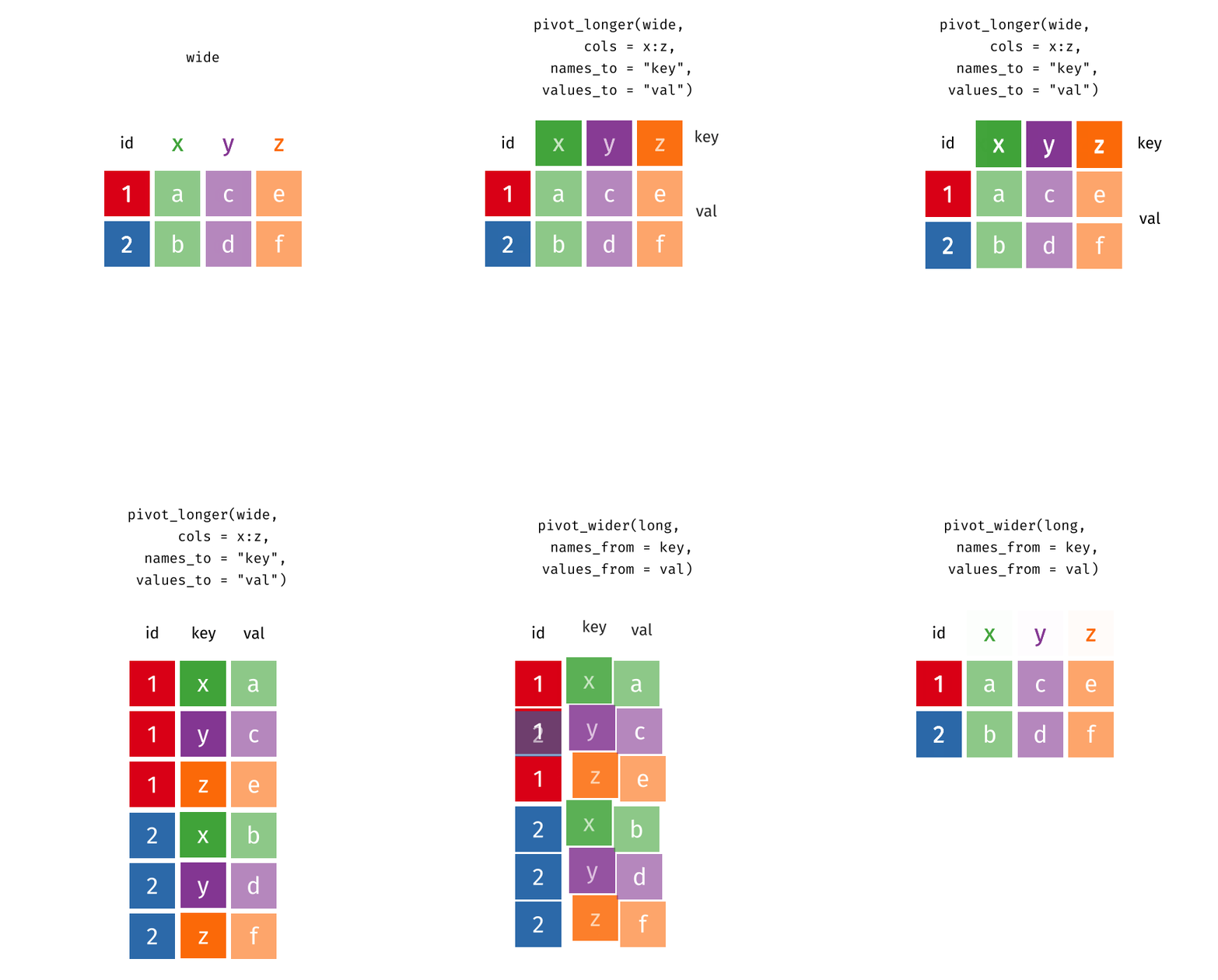
You’ll notice that this format isn’t ideal for data visualization. Columns 5 to 67 represent years, with their values corresponding to life expectancy for each year. However, a cleaner format would be a long data structure, where each row represents a country, a year, and the corresponding life expectancy.
To achieve this, we need to convert the wide format into a long format using the pivot_longer() function.
5.3 Long vs Wide Data
In R, we generally prefer working with the long data (tidy) format for data analysis, as it aligns with the principles of tidy data. A typical tidy dataset follows these rules:
- Each variable has its own column.
- Each observation has its own row.
- Each value has its own cell.
In contrast, wide data format has multiple columns for the same variable, which can make it harder to work with for data analysis and visualization. For example, in this life expectancy dataset, each year is represented as a separate column, however, ideally we want all years to be in a single column named “year”, and all values to be in a single column named “life_expectancy”.
5.4 Transform Wide to Long Data
Let’s check this animation made by Garrick Aden-Buie to understand the transformation from wide to long data format.
# include a gif
knitr::include_graphics("images/tidyr-pivoting.gif")
# Transform wide data to long data format
lifex_long <- lifex |>
  rename(country = `Country Name`,
         country_code = `Country Code`) |>
  pivot_longer(cols = 5:67,
               names_to = "year",
               values_to = "life_expectancy") |>
  mutate(year = as.numeric(year)) |>
select(country, country_code, year, life_expectancy)glimpse(lifex_long)Rows: 16,758
Columns: 4
$ country <chr> "Aruba", "Aruba", "Aruba", "Aruba", "Aruba", "Aruba", …
$ country_code <chr> "ABW", "ABW", "ABW", "ABW", "ABW", "ABW", "ABW", "ABW"…
$ year <dbl> 1960, 1961, 1962, 1963, 1964, 1965, 1966, 1967, 1968, …
$ life_expectancy <dbl> 64.152, 64.537, 64.752, 65.132, 65.294, 65.502, 66.063…summary(lifex_long) country country_code year life_expectancy
Length:16758 Length:16758 Min. :1960 Min. :11.99
Class :character Class :character 1st Qu.:1975 1st Qu.:57.03
Mode :character Mode :character Median :1991 Median :66.96
Mean :1991 Mean :64.39
3rd Qu.:2007 3rd Qu.:72.65
Max. :2022 Max. :85.53
NA's :634 5.5 Merging with World Map Data: mutating join
OK, now we have cleaned up the life expectancy data and transformed it into a long format. Next, we will merge this data with the world map data to prepare for map visualization.
We will load the world map data from the package rnaturalearth, which provides spatial data for countries.
Load World Map Data
world <- ne_countries(scale = "medium", returnclass = "sf") |>
select(iso_a3, geometry)ne_countries() function from the rnaturalearth package returns a spatial feature object with country geometries. ne stands for Natural Earth, which is a public domain map dataset. We select the iso_a3 column as the country code (because it’s in the same format as the country column in the world bank data) and the geometry column for plotting.
Merge Data by left_join()
Then, we will use the left_join() function to merge the life expectancy data with the world map data based on the country_code and iso_a3 columns.
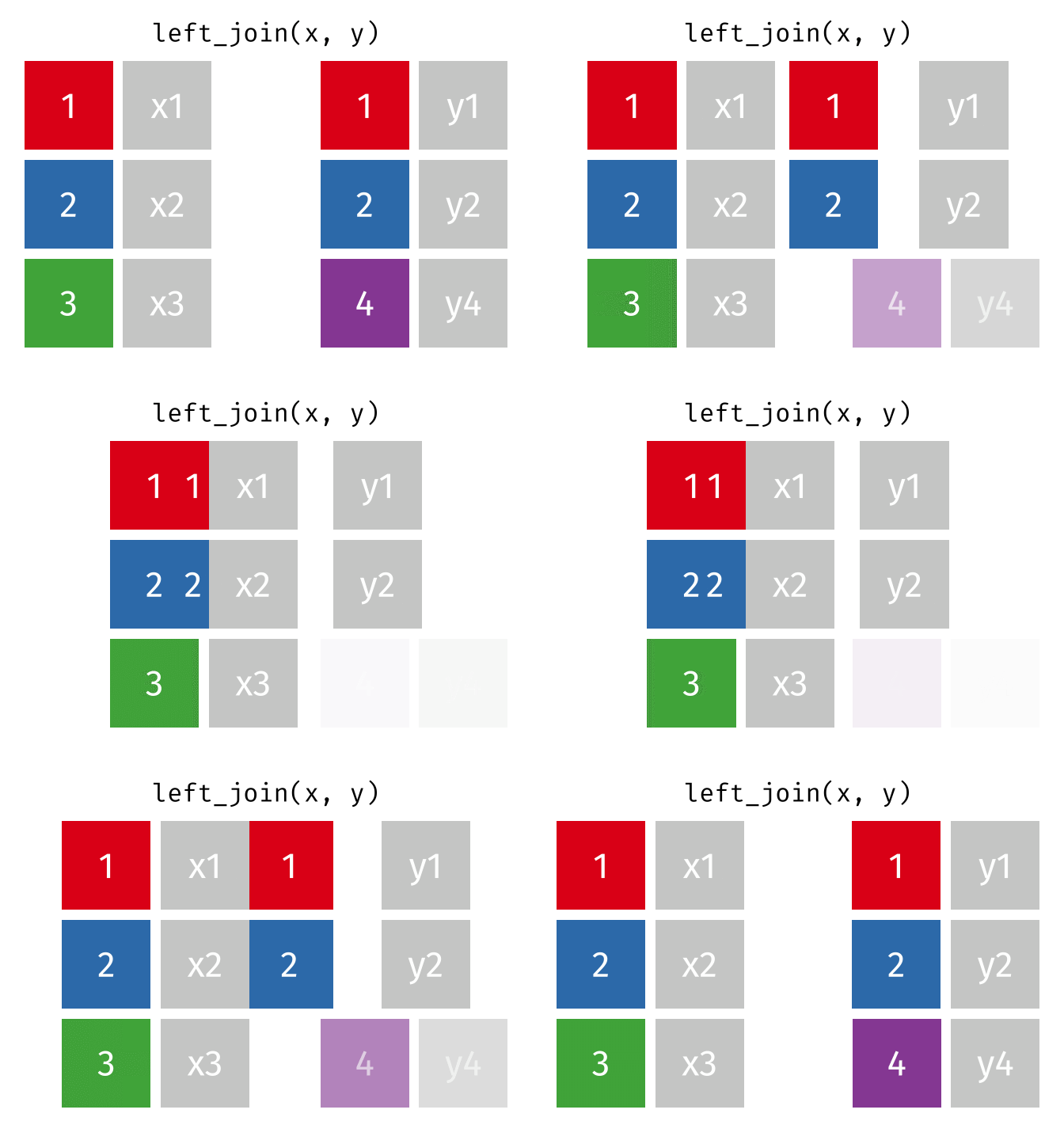
Here is how the left_join() function works (by Garrick Aden-Buie):
knitr::include_graphics("images/left-join.gif")
Here we will use left_join to merge the world map data with the life expectancy data based on the country codes. The reason we let world be the left table is that we want to keep all countries in the world map data, even if they don’t have life expectancy data. Otherwise, we would lose some countries in the map.
# Merge life expectancy data with world map data
df_merge <- lifex_long |>
left_join(world, by = c("country_code" = "iso_a3"))glimpse(df_merge)Rows: 16,758
Columns: 5
$ country <chr> "Aruba", "Aruba", "Aruba", "Aruba", "Aruba", "Aruba", …
$ country_code <chr> "ABW", "ABW", "ABW", "ABW", "ABW", "ABW", "ABW", "ABW"…
$ year <dbl> 1960, 1961, 1962, 1963, 1964, 1965, 1966, 1967, 1968, …
$ life_expectancy <dbl> 64.152, 64.537, 64.752, 65.132, 65.294, 65.502, 66.063…
$ geometry <MULTIPOLYGON [°]> MULTIPOLYGON (((-69.89912 1..., MULTIPOLY…summary(df_merge) country country_code year life_expectancy
Length:16758 Length:16758 Min. :1960 Min. :11.99
Class :character Class :character 1st Qu.:1975 1st Qu.:57.03
Mode :character Mode :character Median :1991 Median :66.96
Mean :1991 Mean :64.39
3rd Qu.:2007 3rd Qu.:72.65
Max. :2022 Max. :85.53
NA's :634
geometry
MULTIPOLYGON :16758
epsg:4326 : 0
+proj=long...: 0
Here we found there are some NAs for year and life_expectancy, which means some countries don’t have life expectancy data in some years.
Clean up NAs and spatial features
library(sf)Linking to GEOS 3.13.0, GDAL 3.8.5, PROJ 9.5.1; sf_use_s2() is TRUEdf_merge <- df_merge |>
filter(!is.na(year) & !is.na(life_expectancy))
# rows number reduced from 16758 to 16124 (there are 634 missing values in life_expectancy column)country_list <- world$iso_a35.6 Save the Merged Data
# Save the merged data to .RData
save(df_merge, file = "out/expectancy_merged.RData")
See Chapter 10 for following data analysis and visualization.
5.7 Key Functions Recap
| Function | Package | Purpose | Example Use |
|---|---|---|---|
pivot_longer() |
tidyr |
Transform wide data to long format | lifex |> pivot_longer(cols = 5:67, names_to = "year", values_to = "life_expectancy") |
left_join() |
dplyr |
Merge datasets keeping all rows from left table | lifex_long |> left_join(world, by = c("country_code" = "iso_a3")) |
ne_countries() |
rnaturalearth |
Load world map spatial data | ne_countries(scale = "medium", returnclass = "sf") |
rename() |
dplyr |
Rename columns in a data frame | rename(country = Country Name, country_code = Country Code) |
select() |
dplyr |
Select specific columns | select(country, country_code, year, life_expectancy) |
filter() |
dplyr |
Filter rows based on conditions | filter(!is.na(year) & !is.na(life_expectancy)) |
is.na() |
Base R | Test for missing values | filter(!is.na(life_expectancy)) |
mutate() |
dplyr |
Create or modify columns | mutate(year = as.numeric(year)) |
save() |
Base R | Save R objects to .RData file | save(df_merge, file = "out/expectancy_merged.RData") |