Appendix D — Final Project Extras

This notebook summarizes some common functions to be used to organize the final project (Quarto Website).

D.1 Data Cleaning

Save Cleaned Data

Suppose you have cleaned your data and stored it in a cleaned version called df_clean. You want to save it as an .RData file for later use.

# Save cleaned data "df_clean" to .RData
save(df_clean, file = "cleaned_data.RData")

D.2 Data Analysis & Visualization

Load Cleaned Data

At the beginning of your analysis, you need to load the cleaned data you saved earlier.

# Load cleaned data
load("cleaned_data.RData")

D.3 Save Plots and Insert in Home Page

Static Plots

Suppose you have created a scatter plot p1 using ggplot2 and want to save it as a PNG file.

# Save plot as PNG
ggsave("out/scatter_plot.png", plot = p1, width = 8, height = 6, dpi = 300)

In your home page, you can insert the saved plot using (no codechunk is needed):

![Scatter Plot](out/scatter_plot.png)

Interactive Plots

Suppose you have created an interactive plot p2 using plotly and want to save it as an HTML file.

library(htmlwidgets) # install if not already installed
htmlwidgets::saveWidget(p2, "out/interactive_plot.html", selfcontained = TRUE)

In your home page, you can insert the saved interactive plot using:

library(htmltools) # install if not already installed
tags$iframe(
src = "out/interactive_plot.html", 
width = "800px", 
height = "600px")

D.4 Arranging Plots

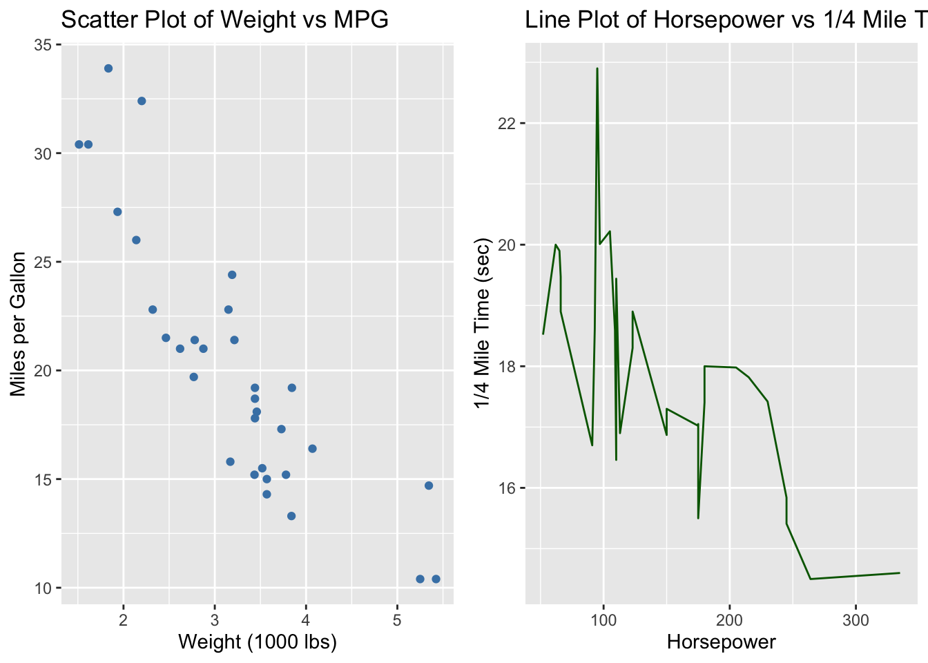
You can also arrange multiple plots in a grid layout using the ggpubr package.

Suppose you have two plots p1 and p2 and want to arrange them in a 1x2 grid.

# Load required libraries
library(ggplot2)
library(ggpubr)

# Use mtcars as the cleaned dataset
df_clean <- mtcars

# Create two plots
p1 <- ggplot(data = df_clean, aes(x = wt, y = mpg)) +
  geom_point(color = "steelblue") +
  labs(title = "Scatter Plot of Weight vs MPG",
       x = "Weight (1000 lbs)", y = "Miles per Gallon")

p2 <- ggplot(data = df_clean, aes(x = hp, y = qsec)) +
  geom_line(color = "darkgreen") +
  labs(title = "Line Plot of Horsepower vs 1/4 Mile Time",
       x = "Horsepower", y = "1/4 Mile Time (sec)")

# Arrange plots in a 1x2 grid
arranged_plot <- ggarrange(p1, p2, ncol = 2, nrow = 1)

arranged_plot