7 Data Analysis II

7.1 Overview

In this chapter, we will use a different dataset to demonstrate the three types of questions that are often asked in journalistic reporting.

About the data

This dataset was downloaded from the World Bank website and saved as a CSV file named life_expectancy.csv, stored in the data folder. The dataset was last updated on March 24, 2025, contains the life expectancy at birth for various countries over the years.

Learning Objectives

This chapter will demonstrate three types of data analysis:

Single Variable Analysis: Analyzing the distribution of global life expectancy.
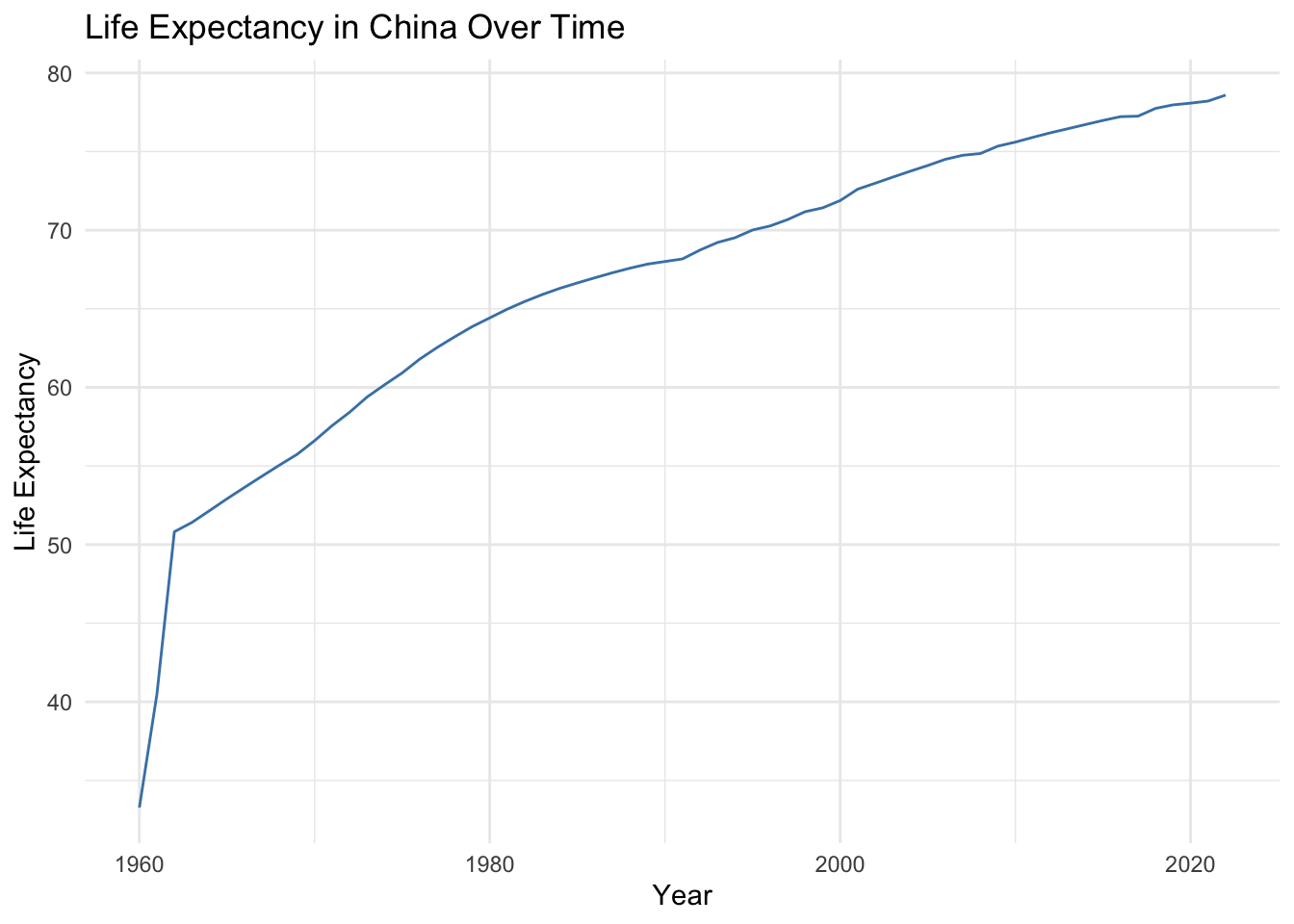
Time-Based Analysis: Tracking changes in China’s life expectancy over time.
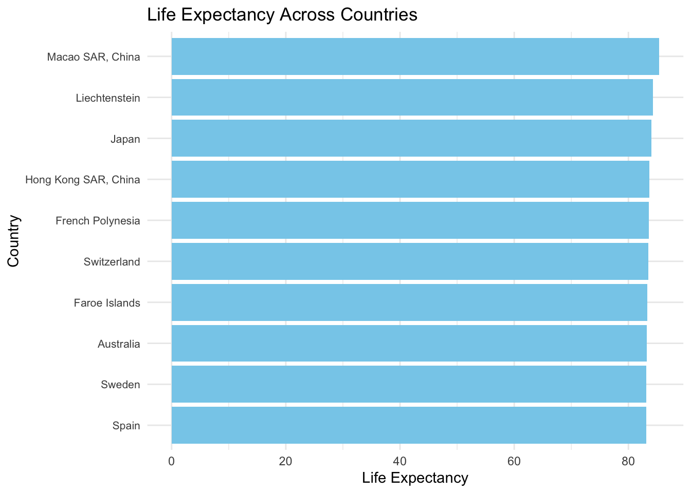
Group Comparisons: Comparing life expectancy across different countries.

7.2 Load data and packages

library(tidyverse)

── Attaching core tidyverse packages ──────────────────────── tidyverse 2.0.0 ──
✔ dplyr     1.1.2     ✔ readr     2.1.4
✔ forcats   1.0.0     ✔ stringr   1.5.0
✔ ggplot2   3.4.2     ✔ tibble    3.2.1
✔ lubridate 1.9.2     ✔ tidyr     1.3.0
✔ purrr     1.0.2     
── Conflicts ────────────────────────────────────────── tidyverse_conflicts() ──
✖ dplyr::filter() masks stats::filter()
✖ dplyr::lag()    masks stats::lag()
ℹ Use the conflicted package (<http://conflicted.r-lib.org/>) to force all conflicts to become errors

lifex <- read_csv("data/life_expectancy.csv")

New names:
Rows: 266 Columns: 69
── Column specification
──────────────────────────────────────────────────────── Delimiter: "," chr
(4): Country Name, Country Code, Indicator Name, Indicator Code dbl (63): 1960,
1961, 1962, 1963, 1964, 1965, 1966, 1967, 1968, 1969, 1970, ... lgl (2): 2023,
...69
ℹ Use `spec()` to retrieve the full column specification for this data. ℹ
Specify the column types or set `show_col_types = FALSE` to quiet this message.
• `` -> `...69`

7.3 Data Wrangling

lifex_clean <- lifex |> 
  select(-`Indicator Name`, -`Indicator Code`, -`Country Code`) |>
  pivot_longer(cols = -`Country Name`, 
               names_to = "year", 
               values_to = "life_expectancy") |>
  mutate(year = as.numeric(year)) |>
  select(country = `Country Name`, year, life_expectancy) |>
  drop_na()

Warning: There was 1 warning in `mutate()`.
ℹ In argument: `year = as.numeric(year)`.
Caused by warning:
! NAs introduced by coercion

glimpse(lifex_clean)

Rows: 16,124
Columns: 3
$ country         <chr> "Aruba", "Aruba", "Aruba", "Aruba", "Aruba", "Aruba", …
$ year            <dbl> 1960, 1961, 1962, 1963, 1964, 1965, 1966, 1967, 1968, …
$ life_expectancy <dbl> 64.152, 64.537, 64.752, 65.132, 65.294, 65.502, 66.063…

7.4 Single Variable Analysis: Understanding Global Life Expectancy Distribution

# Summary statistics of life expectancy
lifex_clean |> 
  summarise(
    avg = mean(life_expectancy, na.rm = TRUE),
    median = median(life_expectancy, na.rm = TRUE),
    min = min(life_expectancy, na.rm = TRUE),
    max = max(life_expectancy, na.rm = TRUE)
  )

# visualize the distribution of life expectancy
hist(lifex_clean$life_expectancy, 
     main = "Global Life Expectancy Distribution",
     xlab = "Life Expectancy",
     col = "skyblue",
     border = "black")

7.5 Time-Based Analysis: Tracking Changes in China’s Life Expectancy

lifex_clean |>
  filter(country == "China") |>
  ggplot(aes(x = year, y = life_expectancy)) +
  geom_line(color = "steelblue") +
  labs(title = "Life Expectancy in China Over Time",
       x = "Year",
       y = "Life Expectancy") +
  theme_minimal()

7.6 Group Comparisons: Comparing Life Expectancy Across Countries

lifex_clean |>
  filter(year == 2022) |>
  top_n(10, life_expectancy) |>
  ggplot(aes(x = reorder(country, life_expectancy), y = life_expectancy)) +
  geom_col(fill = "skyblue") +
  coord_flip() +
  labs(title = "Life Expectancy Across Countries",
       x = "Country",
       y = "Life Expectancy") +
  theme_minimal() +
  theme(axis.text.y = element_text(size = 8))