15  Text Analysis

2024 US Presidential Debate

15.1 Text Analysis with R: 2024 US Presidential Debate

15.2 Load Packages

library(tidyverse)

── Attaching core tidyverse packages ──────────────────────── tidyverse 2.0.0 ──
✔ dplyr     1.1.4     ✔ readr     2.1.5
✔ forcats   1.0.1     ✔ stringr   1.6.0
✔ ggplot2   4.0.0     ✔ tibble    3.3.0
✔ lubridate 1.9.4     ✔ tidyr     1.3.1
✔ purrr     1.2.0     
── Conflicts ────────────────────────────────────────── tidyverse_conflicts() ──
✖ dplyr::filter() masks stats::filter()
✖ dplyr::lag()    masks stats::lag()
ℹ Use the conflicted package (<http://conflicted.r-lib.org/>) to force all conflicts to become errors

library(tidytext)
library(skimr)

15.3 Cleaning Text Data to Data Frame

Import

# Read the transcript
transcript <- readLines("data/debate.txt")
transcript[1:10]

 [1] "PARTICIPANTS:"                                                                                                                                                                                                                                                                                                                      
 [2] "Vice President Kamala Harris (D) and"                                                                                                                                                                                                                                                                                               
 [3] "Former President Donald Trump (R)"                                                                                                                                                                                                                                                                                                  
 [4] ""                                                                                                                                                                                                                                                                                                                                   
 [5] "MODERATORS:"                                                                                                                                                                                                                                                                                                                        
 [6] "Linsey Davis (ABC News) and"                                                                                                                                                                                                                                                                                                        
 [7] "David Muir (ABC News)"                                                                                                                                                                                                                                                                                                              
 [8] ""                                                                                                                                                                                                                                                                                                                                   
 [9] "MUIR: Good evening, I'm David Muir. And thank you for joining us for tonight's ABC News Presidential Debate. We want to welcome viewers watching on ABC and around the world tonight. Vice President Kamala Harris and President Donald Trump are just moments away from taking the stage in this unprecedented race for president."
[10] ""                                                                                                                                                                                                                                                                                                                                   

# Remove empty lines
transcript <- transcript[transcript != ""]

Parse transcripts to a data frame

# Initialize an empty data frame
data <- data.frame(speaker = character(),
                   text = character(),
                   stringsAsFactors = FALSE)

# Define a regular expression pattern to detect speaker lines
speaker_pattern <- "^[A-Z ]+:"  # Lines that start with uppercase letters followed by a colon
# Initialize variables
current_speaker <- NA
current_text <- ""

for (line in transcript) {
  # Check if the line matches the speaker pattern
  if (str_detect(line, speaker_pattern)) {
    # If there's accumulated text, save it before moving to the next speaker
    if (!is.na(current_speaker) && current_text != "") {
      data <- rbind(data, data.frame(speaker = current_speaker, text = current_text, stringsAsFactors = FALSE))
      current_text <- ""
    }
    # Extract the speaker
    split_line <- str_split_fixed(line, ":", 2)
    current_speaker <- str_trim(split_line[1])
    # Start accumulating text
    current_text <- str_trim(split_line[2])
  } else {
    # Accumulate text
    current_text <- paste(current_text, str_trim(line))
  }
}

# Add the last piece of text
if (!is.na(current_speaker) && current_text != "") {
  data <- rbind(data, data.frame(speaker = current_speaker, text = current_text, stringsAsFactors = FALSE))
}

# write_csv(data, "out/debate_df.csv")

15.4 Import Cleaned Data

df <- data

skim(df)

Data summary

Name	df
Number of rows	230
Number of columns	2
_______________________
Column type frequency:
character	2
________________________
Group variables	None

Variable type: character

skim_variable	n_missing	complete_rate	min	max	empty	n_unique	whitespace
speaker	0	1	4	12	0	6	0
text	0	1	8	2361	0	219	0

unique(df$Speaker)

NULL

15.5 Data Cleaning

Filter Out Non-Candidate Speakers

df1 <- df |>
  filter(speaker == "HARRIS" | speaker == "TRUMP")

unique(df1$speaker)

[1] "HARRIS" "TRUMP" 

Standardize Speaker Names

# Standardize speaker names if necessary
df1$speaker <- ifelse(df1$speaker == "HARRIS", "Harris", "Trump")

15.6 Text Analysis

Tokenize and Remove Stop Words

# Tokenize the text column
tidy_data <- df1 %>%
  unnest_tokens(word, text)

head(tidy_data)

# Load stop words
data("stop_words")

# Remove stop words
tidy_data_clean <- tidy_data %>%
  anti_join(stop_words, by = "word") %>%
  filter(!str_detect(word, "\\d+"))

# Calculate word frequencies
word_counts <- tidy_data_clean %>%
  count(speaker, word, sort = TRUE)

Analyze Top Words

# Get top 10 words for each candidate
top_words <- word_counts %>%
  group_by(speaker) %>%
  top_n(10, n) %>%
  ungroup() %>%
  arrange(speaker, -n)

# View the result
print(top_words)

# A tibble: 22 × 3
   speaker word           n
   <chr>   <chr>      <int>
 1 Harris  president     56
 2 Harris  people        48
 3 Harris  donald        32
 4 Harris  trump         31
 5 Harris  american      27
 6 Harris  united        21
 7 Harris  plan          20
 8 Harris  understand    18
 9 Harris  care          14
10 Harris  talk          14
# ℹ 12 more rows

Analyze Top Word Pairs (Bigrams)

# Create bigrams
bigrams <- df1 %>%
  unnest_tokens(bigram, text, token = "ngrams", n = 2)

# Separate bigrams into two words
bigrams_separated <- bigrams %>%
  separate(bigram, into = c("word1", "word2"), sep = " ")

# Remove stop words
bigrams_filtered <- bigrams_separated %>%
  filter(!word1 %in% stop_words$word,
         !word2 %in% stop_words$word) %>%
  # remove numbers 
  filter(!str_detect(word1, "\\d+"),
         !str_detect(word2, "\\d+"))

# Unite the words back into bigrams
bigram_counts <- bigrams_filtered %>%
  unite(bigram, word1, word2, sep = " ") %>%
  count(speaker, bigram, sort = TRUE)

# Get top 10 bigrams for each candidate
top_bigrams <- bigram_counts %>%
  group_by(speaker) %>%
  top_n(10, n) %>%
  ungroup() %>%
  arrange(speaker, -n)

# View the result
print(top_bigrams)

# A tibble: 23 × 3
   speaker bigram                n
   <chr>   <chr>             <int>
 1 Harris  donald trump         26
 2 Harris  american people      18
 3 Harris  vice president       11
 4 Harris  affordable care       7
 5 Harris  care act              7
 6 Harris  donald trump's        6
 7 Harris  health care           5
 8 Harris  middle class          5
 9 Harris  national security     5
10 Harris  trump left            4
# ℹ 13 more rows

15.7 Plot

Top words

# Plot
top_words %>%
  mutate(word = reorder_within(word, n, speaker)) %>%
  ggplot(aes(word, n, fill = speaker)) +
  geom_col(show.legend = FALSE) +
  facet_wrap(~speaker, scales = "free_y") +
  coord_flip() +
  scale_x_reordered() +
  labs(x = "Words", y = "Frequency", title = "Top Words by Candidate")

Top Bigrams

# Plot
top_bigrams %>%
  mutate(bigram = reorder_within(bigram, n, speaker)) %>%
  ggplot(aes(bigram, n, fill = speaker)) +
  geom_col(show.legend = FALSE) +
  facet_wrap(~speaker, scales = "free_y") +
  coord_flip() +
  scale_x_reordered() +
  labs(x = "Bigrams", y = "Frequency", title = "Top Bigrams by Candidate")

15.8 Word Cloud

library(wordcloud)

Loading required package: RColorBrewer

library(RColorBrewer)

# Filter word counts for each candidate
harris_words <- word_counts %>%
  filter(speaker == "Harris")

trump_words <- word_counts %>%
  filter(speaker == "Trump")

Single Plot

wordcloud(words = harris_words$word, 
          freq = harris_words$n, 
          min.freq = 2,
          max.words = 100,
          random.order = FALSE, 
          rot.per = 0.35, 
          colors = brewer.pal(8, "Blues"),
          scale = c(4, 0.5))
title("Harris")

Side-by-Side

# Set up the plotting area for two plots
par(mfrow = c(1, 2))

# Word cloud for Harris
wordcloud(words = harris_words$word, 
          freq = harris_words$n, 
          min.freq = 2,
          max.words = 100,
          random.order = FALSE, 
          rot.per = 0.35, 
          colors = brewer.pal(8, "Blues"),
          scale = c(4, 0.5))

Warning in wordcloud(words = harris_words$word, freq = harris_words$n, min.freq
= 2, : people could not be fit on page. It will not be plotted.

Warning in wordcloud(words = harris_words$word, freq = harris_words$n, min.freq
= 2, : manufacturing could not be fit on page. It will not be plotted.

Warning in wordcloud(words = harris_words$word, freq = harris_words$n, min.freq
= 2, : taliban could not be fit on page. It will not be plotted.

Warning in wordcloud(words = harris_words$word, freq = harris_words$n, min.freq
= 2, : understands could not be fit on page. It will not be plotted.

Warning in wordcloud(words = harris_words$word, freq = harris_words$n, min.freq
= 2, : zelenskyy could not be fit on page. It will not be plotted.

title("Harris")

# Word cloud for Trump
wordcloud(words = trump_words$word, 
          freq = trump_words$n, 
          min.freq = 2,
          max.words = 100,
          random.order = FALSE, 
          rot.per = 0.35, 
          colors = brewer.pal(8, "Reds"),
          scale = c(4, 0.5))
title("Trump")

15.9 Compare on fixed categories

# Define the list of agenda keywords
agenda_keywords <- c("border", "abortion", "economy", "immigration", "health", "security", "israel", "russia", "china", "ukraine")

# Convert words to lowercase
tidy_data_clean <- tidy_data_clean %>%
  mutate(word = tolower(word))

# Filter words that are in the agenda_keywords list
agenda_data <- tidy_data_clean %>%
  filter(word %in% agenda_keywords)

# Count the frequency of each keyword per candidate
agenda_counts <- agenda_data %>%
  count(speaker, word) %>%
  arrange(speaker, desc(n))

print(agenda_counts)

   speaker        word  n
1   Harris    security  9
2   Harris     economy  8
3   Harris    abortion  6
4   Harris      health  6
5   Harris      israel  5
6   Harris     ukraine  5
7   Harris      border  3
8   Harris       china  3
9   Harris      russia  2
10  Harris immigration  1
11   Trump     economy 13
12   Trump      border 11
13   Trump       china 10
14   Trump    abortion  8
15   Trump      russia  8
16   Trump      israel  7
17   Trump     ukraine  6
18   Trump      health  2
19   Trump immigration  2
20   Trump    security  2

15.10 Heatmap

# Create a heatmap
ggplot(agenda_counts, aes(x = word, y = speaker, fill = n)) +
  geom_tile() +
  scale_fill_gradient(low = "white", high = "red") +
  labs(title = "Agenda Keyword Frequencies Heatmap",
       x = " ",
       y = " ") +
  theme_minimal() +
  # remove grid
  theme(panel.grid.major = element_blank(),
        panel.grid.minor = element_blank()
        )

15.11 Key Functions Recap

Function	Package	Purpose	Example Use
readLines()	Base R	Read lines from a text file	readLines("data/debate.txt")
str_detect()	stringr	Detect pattern matching in strings	str_detect(line, speaker_pattern)
str_split_fixed()	stringr	Split string into fixed number of pieces	str_split_fixed(line, ":", 2)
str_trim()	stringr	Remove leading/trailing whitespace	str_trim(split_line[1])
rbind()	Base R	Bind rows of data frames together	rbind(data, data.frame(speaker = current_speaker, text = current_text))
skim()	skimr	Quick data summary and exploration	skim(df)
unique()	Base R	Extract unique values	unique(df$speaker)
filter()	dplyr	Filter rows based on conditions	filter(speaker == "HARRIS" \| speaker == "TRUMP")
ifelse()	Base R	Vector conditional function	ifelse(df1$speaker == "HARRIS", "Harris", "Trump")
unnest_tokens()	tidytext	Tokenize text into individual words	unnest_tokens(word, text)
anti_join()	dplyr	Keep rows not matching another table	anti_join(stop_words, by = "word")
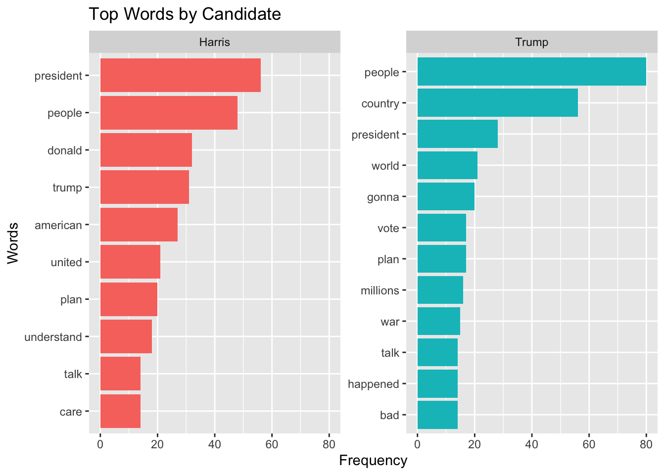
count()	dplyr	Count occurrences of unique values	count(speaker, word, sort = TRUE)
group_by()	dplyr	Group data by one or more variables	group_by(speaker)
top_n()	dplyr	Select top n rows by value	top_n(10, n)
ungroup()	dplyr	Remove grouping from data frame	ungroup()
arrange()	dplyr	Sort rows by one or more columns	arrange(speaker, -n)
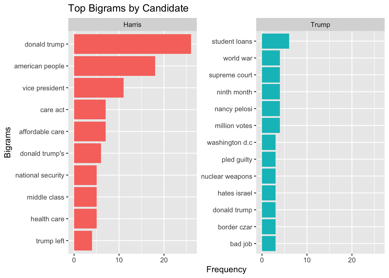
separate()	tidyr	Separate a column into multiple columns	separate(bigram, into = c("word1", "word2"), sep = " ")
unite()	tidyr	Unite multiple columns into one	unite(bigram, word1, word2, sep = " ")
mutate()	dplyr	Create or modify columns	mutate(word = tolower(word))
tolower()	Base R	Convert strings to lowercase	tolower(word)
reorder_within()	tidytext	Reorder factor within groups for visualization	reorder_within(word, n, speaker)
ggplot()	ggplot2	Create a new ggplot object	ggplot(aes(word, n, fill = speaker))
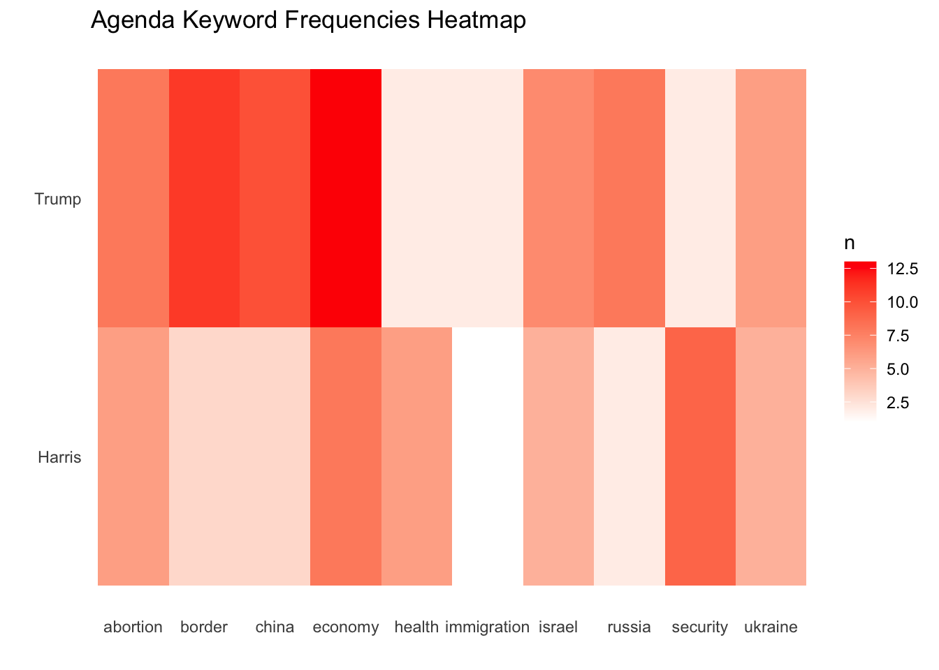
aes()	ggplot2	Specify aesthetic mappings (x, y, color, fill)	aes(x = word, y = speaker, fill = n)
geom_col()	ggplot2	Create a bar chart	geom_col(show.legend = FALSE)
geom_tile()	ggplot2	Create a heatmap (tile plot)	geom_tile()
facet_wrap()	ggplot2	Create multiple plots based on categorical var	facet_wrap(~speaker, scales = "free_y")
coord_flip()	ggplot2	Flip x and y axes	coord_flip()
scale_x_reordered()	tidytext	Apply reordered scale to x-axis	scale_x_reordered()
scale_fill_gradient()	ggplot2	Create gradient color scale for fill	scale_fill_gradient(low = "white", high = "red")
labs()	ggplot2	Add titles, labels, and captions	labs(title = "...", x = "Words", y = "Frequency")
theme_minimal()	ggplot2	Apply minimal theme	theme_minimal()
element_blank()	ggplot2	Create blank (invisible) element	element_blank()
theme()	ggplot2	Customize plot appearance	theme(panel.grid.major = element_blank())
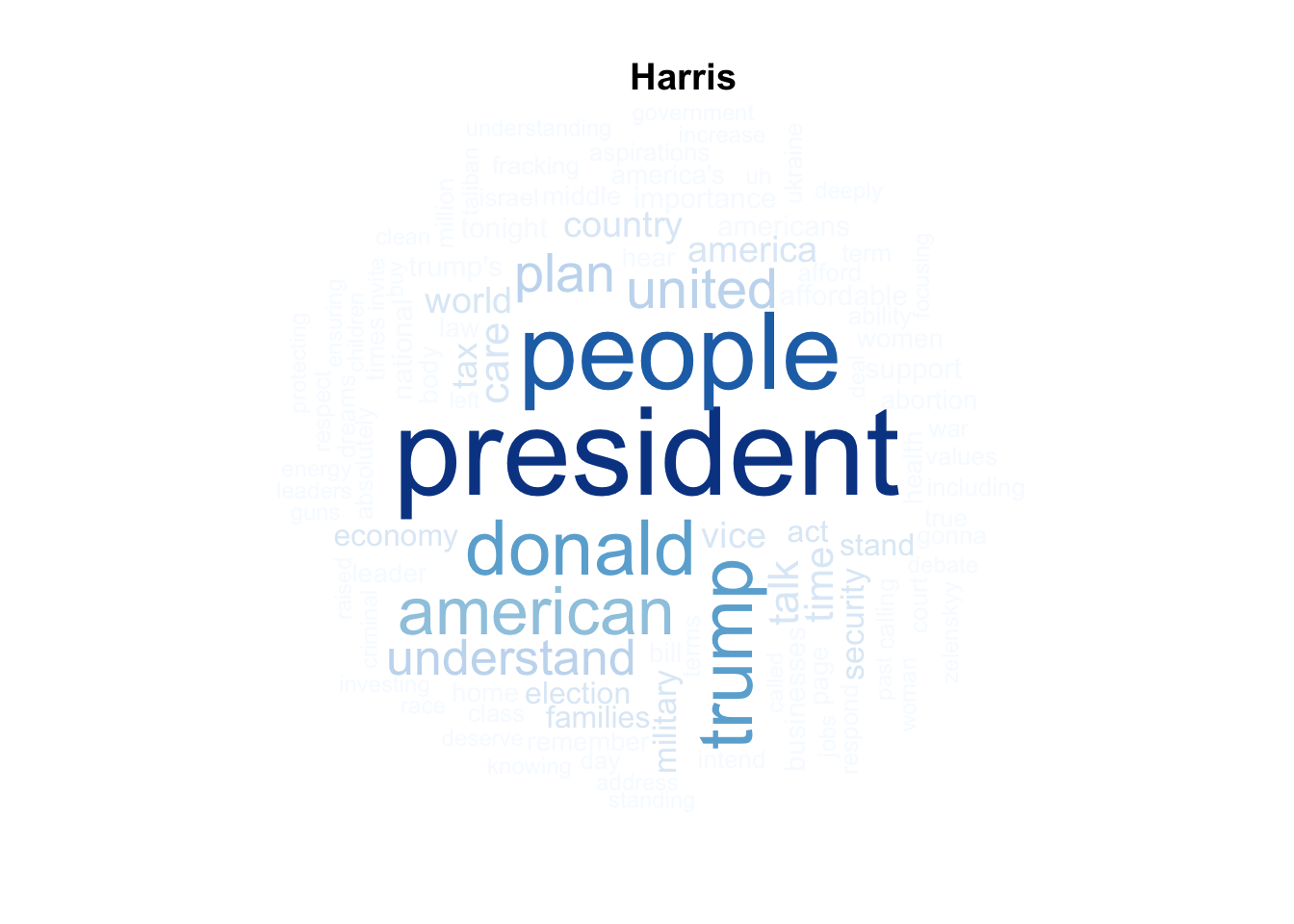
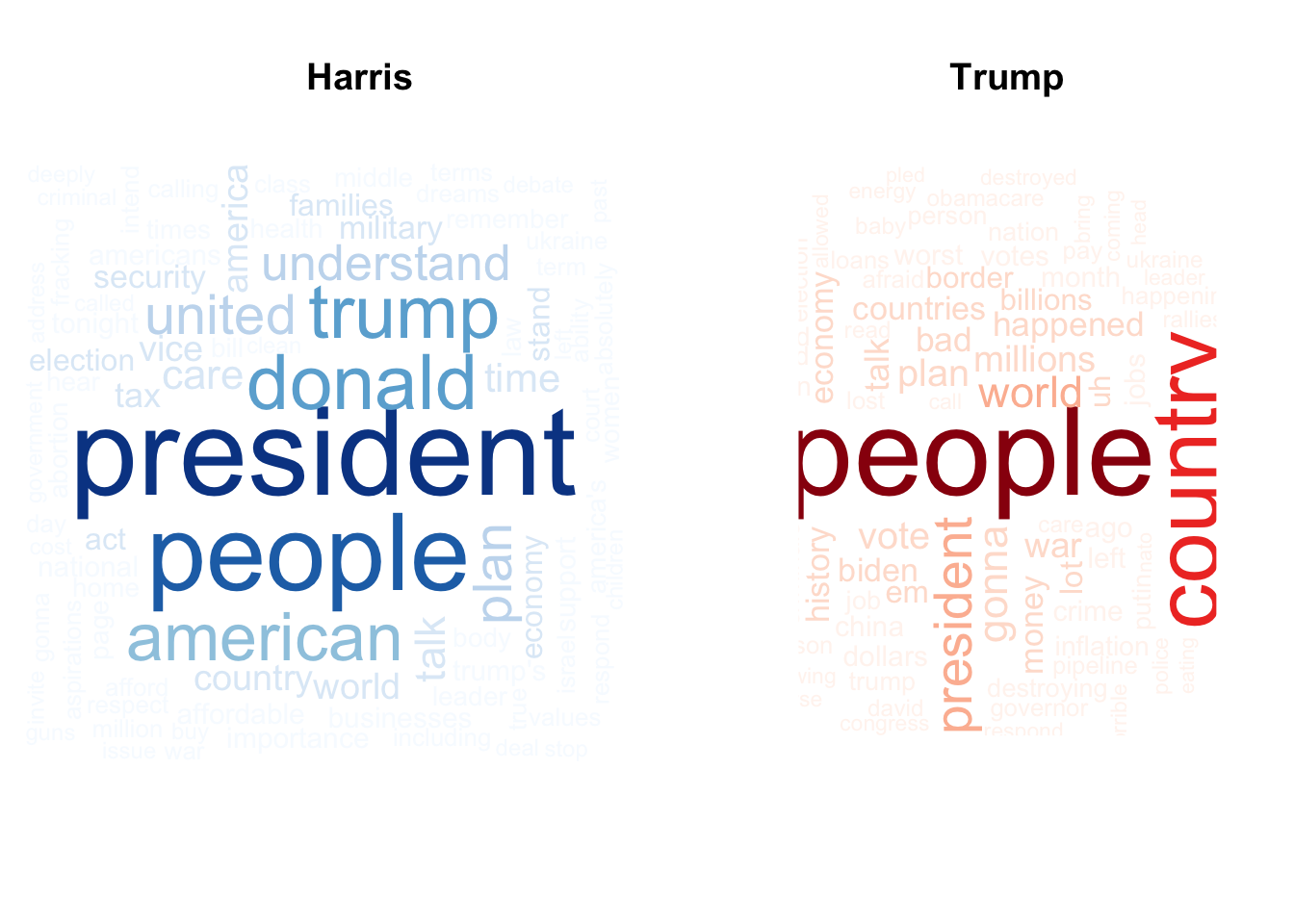
wordcloud()	wordcloud	Create a word cloud visualization	wordcloud(words = harris_words$word, freq = harris_words$n, max.words = 100)
brewer.pal()	RColorBrewer	Generate color palettes	brewer.pal(8, "Blues")
par()	Base R	Set or query graphical parameters	par(mfrow = c(1, 2))
data()	Base R	Load built-in datasets	data("stop_words")