1 Installation & Setup
Part 1: Getting Started
Before you can analyze data, you need to set up your tools. This part walks you through installation and introduces R basics—the foundation for everything that follows.
What you’ll learn: - Install R and RStudio on your computer - Understand basic R syntax and how code works - Work with variables, functions, and data types - Run your first data analysis
Don’t rush these chapters. A solid foundation makes the rest of the book much easier.
1.1 Why Learn R for Data Journalism?
Data journalism requires tools that combine statistical rigor with storytelling capabilities. R provides:
- Reproducible analysis through script-based workflows
- Advanced visualization for impactful storytelling
- Open-source community with continuous innovation
- Professional-grade tools used by NYT, BBC, and Reuters etc.
1.2 Installing the Tools
Step 1: Install R
- Visit CRAN Mirror
- Select your operating system (Windows/Mac/Linux)
- Download the latest version (≥4.3.0 recommended)
- Run the installer with default settings
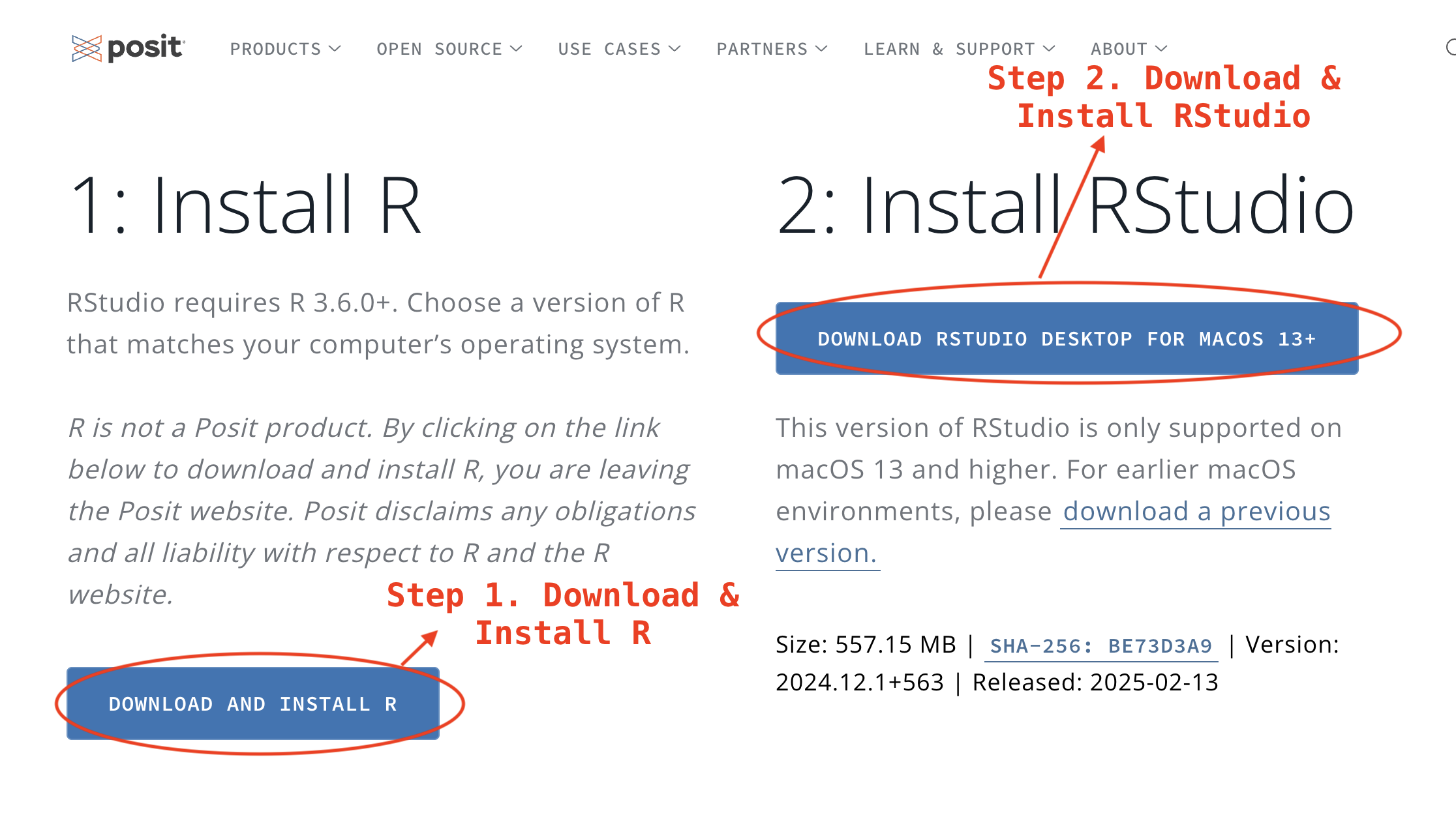
Step 2: Install RStudio
- Go to posit.co/download
- Choose Download RStudio Desktop
- Install using default options
Important
Installation Order Matters! Always install R before RStudio - the IDE needs the base R engine to function.
1.3 First-Time Setup
Organizing Your Workspace
Create a project folder:
- Windows:
C:/Users/[YourName]/Documents/djr - Mac:
/Users/[YourName]/Documents/djr
- Windows:
Use lowercase letters only (avoid spaces/special characters)
# Create folder from R Console (alternative method)
dir.create("~/Documents/djr")
Configuring RStudio
Optimize your setup through:
- Tools > Global Options > General
- Uncheck everything above the “Other” panel
- Set “Save workspace” to Never
- Tools > Global Options > Code
- Enable “Soft-wrap R source files”
- Check “Use native pipe operator |>”
1.4 Understanding the RStudio Interface
| Position | Panel | Purpose | Key Features |
|---|---|---|---|
| Top-Left | Source | Code editing | Scripts, R Markdown, notebooks |
| Bottom-Left | Console | Direct code execution | Immediate feedback, debugging |
| Top-Right | Environment | Active data objects | Variable inspection |
| Bottom-Right | Files/Help | Navigation & documentation | Package help, file browsing |
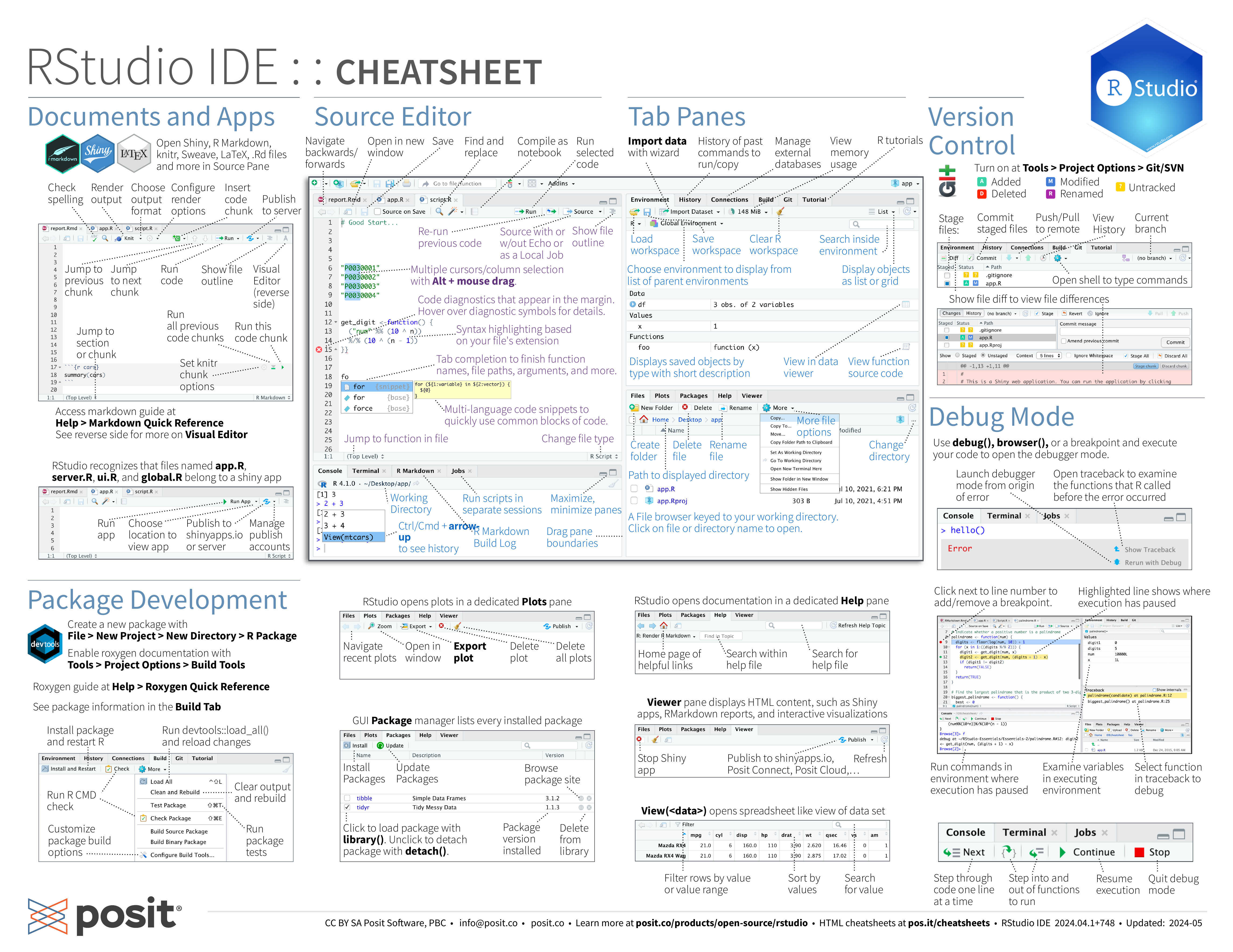
Download full RStudio IDE cheatsheets
1.5 Essential Packages Installation
Run this in the Console:
install.packages(c(
  "tidyverse",   # Data wrangling & visualization
  "rmarkdown",   # Dynamic reporting
  "quarto",      # Modern publishing
  "knitr",       # Document processing
  "janitor"      # Data cleaning
))
1.6 Your First Project
Create an R Project
- File > New Project > New Directory
- Name:
yourname-week1(e.g.,bin-week1) - Browse to your
djrfolder - Click Create Project
Once created, your project folder will be the “main workspace” for all your work. Keep all your scripts, data, and outputs organized here. This is essential for reproducibility and managing your workflow.
Create Your First Document
- File > New File > R Markdown (or Quarto document)
- Title: “My First Analysis”
- Author: Your Name
- Default HTML output
- Save the file as
analysis.Rmd
Quick Test
Now that you have a fresh R Markdown document, test that everything works:
- Replace the template content with:
# Load the tidyverse package
library(tidyverse)

# Create a simple dataset
data <- data.frame(
  publication = c("NYT", "BBC", "Reuters"),
  readers = c(150000, 200000, 120000)
)

# View the data
data- Click Render to generate the output.
If everything works, congratulations! You’re ready for data analysis.
Warning
If you get an error, make sure you: - Installed R and RStudio (in that order) - Installed the tidyverse package via install.packages("tidyverse") in the Console - Used library() (not install.packages()) inside your document
1.7 Writing Your First Document
R Markdown (or Quarto) files combine text, code, and output in a single document. Here’s the basic structure:
YAML Metadata (Document Header)
The top of your file defines settings:
---
title: "Data Journalism"
subtitle: "Week 1"
author: "Bin Chen"
date: "Jan 20, 2025"
format: html
---
Text & Code
Write narrative using regular text and Markdown formatting: - **bold** for bold text - # Heading for section headers - - item for lists - [link text](url) for links
Insert R code using code chunks:
# Your R code goes here
1 + 1
Insert a code chunk with Ctrl + Alt + I (Windows) or Cmd + Option + I (Mac).
Render the Document
Click Render (or Knit in older R Markdown) to generate the output. R will run all code chunks and create an HTML file.
Tip
Never run install.packages() inside your document. Always run package installation in the Console first, then use library() in your document to load it.
1.8 Next Steps
You now have R, RStudio, and the essential packages installed. You’re ready to start learning R basics and analyzing data for journalism.
Move on to the next chapter: R Coding Basics.
2 Key Functions and Shortcuts
| Functionality | Shortcut/Command | Purpose |
|---|---|---|
| Insert code chunk (Windows) | Ctrl + Alt + I |
Add R code to document |
| Insert code chunk (Mac) | Cmd + Option + I |
Add R code to document |
| Install packages | install.packages("package_name") |
install.packages("tidyverse") |
| Load packages | library(package_name) |
library(tidyverse) |
| Render document | Click Render button | Generate HTML/PDF output |
| Get help on function | ?function_name |
?mean |
| View workspace | ls() |
List all objects in memory |